Arrhenius Reparameterization: Same Data, Better-Posed Parameters

Why A and Ea come out almost perfectly correlated in the standard Arrhenius fit, and how a reference temperature, chosen with the Jacobian's help, removes the correlation without adding a single run.

The chemical engineering literature often uses a reparameterized Arrhenius expression, written around a reference temperature. As someone trained in organic and medicinal chemistry, I hadn’t come across it before. This article explains the advantages of the reparameterization (G. E. P. Box, “Fitting empirical data,” Ann. N.Y. Acad. Sci. 86, 792–816, 1960).

The example here is simulated so the true answer is known: Ea = 80 kJ/mol, k = 0.01 s⁻¹ at 70 °C, duplicate runs at 50, 60, 70, 80 and 90 °C. Observed rate constants were simulated as kᵢ = A exp(−Eₐ/(R Tᵢ)) + εᵢ, where the εᵢ are additive IID errors drawn from N(0, σ²). Fitted in the standard form, k = A·exp(−Ea/RT), with NonlinearModelFit, the estimates of A and Ea are correlated at ρ = +0.99986 (the two sensitivity columns have cosine −0.99986). To four decimal places the data cannot tell a high-A, high-Ea pair from a low-A, low-Ea one.

Highly correlated parameters

For a single response, least squares sees the parameters through the Jacobian J: one row per run, one column per parameter, each entry ∂k/∂θ at the optimum. Wolfram gives it symbolically in a couple of lines:

modelStd = A Exp[-Ea/(R T)];
modelRef = kr Exp[-(Ea/R) (1/T - 1/TR)];

D[modelStd, {{A, Ea}}] // Simplify   (* {k/A, -k/(R T)} *)
D[modelRef, {{kr, Ea}}] // Simplify  (* {k/kref, -k (1/T - 1/TR)/R} *)

In the standard form, the sensitivity to A is k/A and the sensitivity to Ea is −k/(RT). Their ratio, −A/(RT), is nearly constant over the experiment, because the absolute temperature only runs from 323 K to 363 K. So the two columns are nearly proportional. Normalized to unit length, they are 0.95° apart:

Two panels of normalized sensitivity versus temperature. Standard form: the curves for ∂k/∂A and −∂k/∂Ea coincide. Centered form: ∂k/∂kref rises steadily while −∂k/∂Ea rises, then turns over and goes negative at 90 °C. — Fig. 1. The two columns of J, evaluated at the least-squares optimum and each scaled to unit length. Standard form: indistinguishable. Centered form: the sensitivity to Ea changes sign near Tref, which makes it orthogonal to the sensitivity to kref.

The information matrix JᵀJ (with Cov(θ) ≈ σ²(JᵀJ)⁻¹) inherits this. Its eigenvalues measure how well the data determine each direction in parameter space. A tiny eigenvalue means a long axis of the confidence region, and the ratio of the largest to the smallest, the condition number, summarizes the problem.

A note on scaling

Raw JᵀJ is not useful for this question. A is about 10¹⁰ s⁻¹ and Ea about 10⁵ J/mol, so the two columns differ by many orders of magnitude, and the raw condition numbers (5.5×10¹⁶ standard, 2.2×10¹³ centered) mostly reflect units. The columns have to be put on a common scale first, and this page uses two scalings:

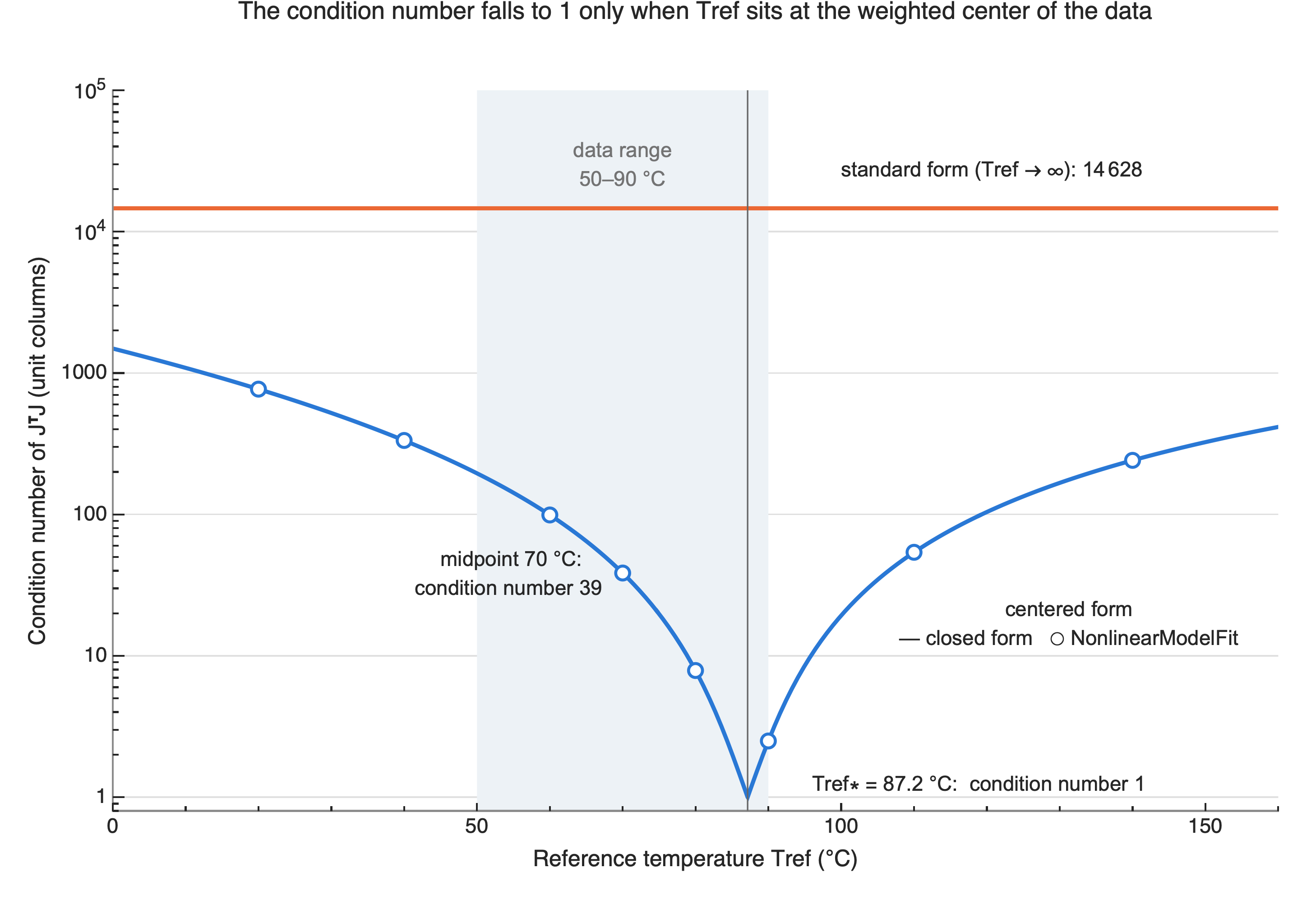
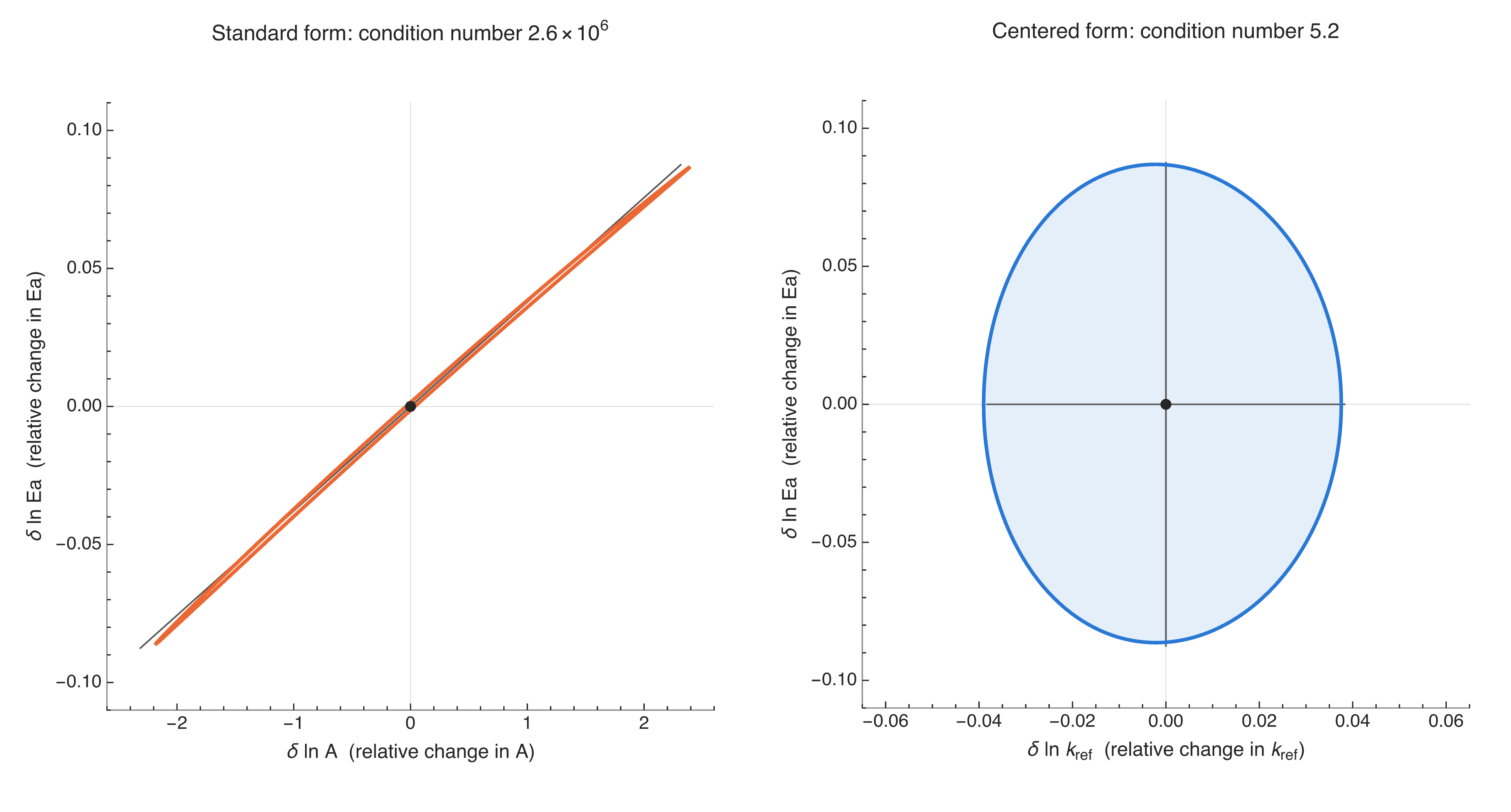
Unit-length columns (Fig. 2). JᵀJ becomes the matrix of cosines between the columns, {{1, c}, {c, 1}}, with eigenvalues 1 ± |c|. For the standard form, c = −0.99986 gives eigenvalues 1.99986 and 0.000137: condition number 14,628.
Relative sensitivities, θⱼ·∂k/∂θⱼ (Fig. 3), which put both axes in “fractional change” units so the confidence regions can be drawn on the same footing. On this scaling the condition numbers are 2.6×10⁶ vs 5.2.

Both scalings tell the same story. The numbers differ because they answer slightly different questions, so don’t compare a number from one with a number from the other.

Centering the temperature

Rewrite the model around a reference temperature:

k = k_ref·exp[−(Ea/R)(1/T − 1/T_ref)]

It’s the same curve and the same fit quality, with k_ref replacing A as the rate constant at T_ref. The sensitivity of k to Ea (the second column of J) is now −k(1/T − 1/T_ref)/R, which changes sign at T_ref. The two columns are orthogonal when 1/T_ref is the k²-weighted mean of 1/T.

The weights matter. With constant absolute error, the fast hot runs dominate the fit, so the optimal reference here is 360.3 K (87.2 °C), not the 70 °C midpoint. At 87.2 °C the condition number is exactly 1. At the midpoint it is still about 39:

Log-scale plot of condition number versus reference temperature from 0 to 160 °C. The centered form dips to 1 at 87.2 °C, reads 39 at 70 °C, and rises on either side. A flat line at 14,628 marks the standard form. Open circles from NonlinearModelFit refits sit on the closed-form curve. — Fig. 2. Condition number of JᵀJ (unit columns) as a function of Tref. The standard form is the Tref → ∞ limit. The open circles are independent NonlinearModelFit refits and land on the closed-form curve.

Results: same information, different shape

The relative-sensitivity JᵀJ has the same determinant for both forms (6.47×10⁻⁶). Going from (ln A, ln Ea) to (ln k_ref, ln Ea) is a shear with unit determinant, so the total information the data carry, which corresponds to the area of the confidence region, is unchanged. What changes is the shape. A thin diagonal needle with axes in the ratio 1601 : 1 becomes an axis-aligned ellipse at 2.3 : 1:

Two joint 95% confidence regions in relative-change coordinates. Left, standard form: a needle-thin diagonal region spanning about ±240% in A. Right, centered form: an ellipse with axes along the parameter axes, spanning about ±4% in kref. — Fig. 3. Exact joint 95% confidence regions, with the eigenvectors of the relative-sensitivity JᵀJ drawn as axes. The two regions have the same area to within 1%. Note the x-axis ranges: about ±240% in A versus about ±4% in kref.

Takeaway

The A–Ea correlation is a property of how the model is written, not a shortage of data. The Jacobian shows it (two nearly parallel columns), the eigensystem of JᵀJ names the unresolvable direction, and a reference temperature at the k²-weighted center of 1/T removes it while leaving the information content untouched.

In practice this is relevant beyond Arrhenius reparameterization. A well-conditioned parameterization makes NonlinearModelFit converge faster and more reliably from rough starting values.

Get in touch if you would like a copy of the Wolfram notebook.

Related: Multiresponse Parameter Estimation: The α-Pinene Kinetics Case Study, another kinetics fit where an eigen-decomposition pinpoints the poorly identified direction in parameter space.